| Home | Notes | Github |
|---|
Written: 17-Jul-2024
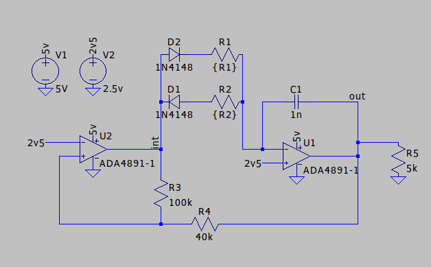
So, something I’m working on requires a sawtooth generator. I did the usual and found a circuit online and got a circuit, fired up LTSpice. Lo and behold it worked!1 Now, how to get the right sawtooth.

One option was to do the maths, but that’s what computers are for.
So I parameterised2 the model, and got it to spew some output. Unfortunately LTSpice meas statements don’t output to a nice .csv file3, but we can smash together some python to do that. Or do one better and keep it in python, and perform some analysis there.
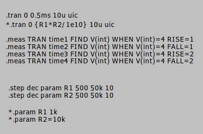
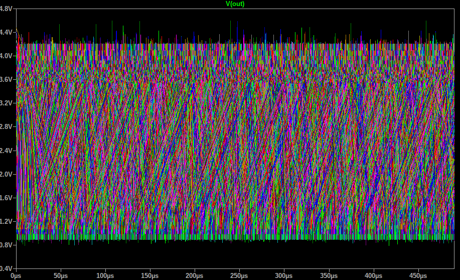
The model swept through different values of R1 and R2 measuring the times of crossing points. The downside of this was getting the run time of the simulation right, because enough low frequency waves took ages to simulate the high frequency waves. But it’s not so important, because I was sleeping 😴.
The results are two nice graphs. First up is the frequency plot. The frequency I need is 37.9kHz, which is highlighted as a red contour. 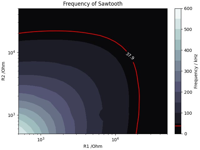
Unsurprisingly the frequency jumps as the resistances go down. What’s surprising is quite how rapidly this occurs. There’s also a weird occlusion around the (7k,1k) point, but that might just be an artefact of how many points we have.
Next the duty ratio required is 0.12. Again, same drill as the previous plot.
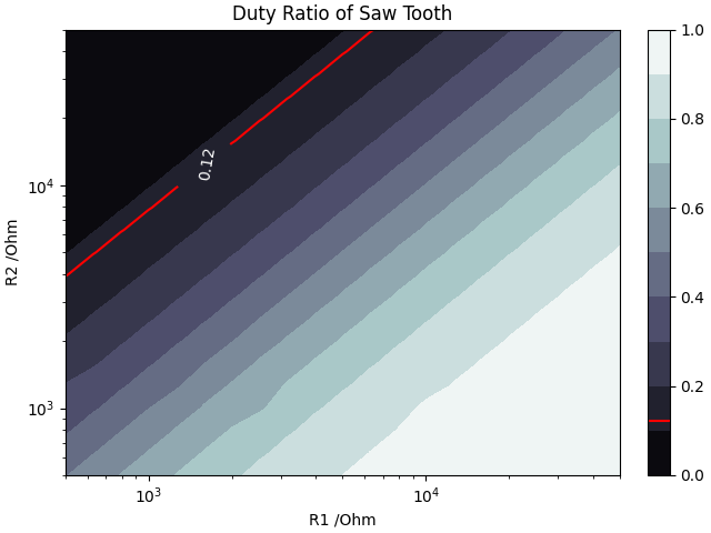 This plot is a bit more expected, and it’s purely a ratio of the two resistor values. However, given this was almost4 free, and I didn’t know for sure that it’s how it would behave, it was worth doing that bit of faff. Plus it allows me to see where those two lines overlap!
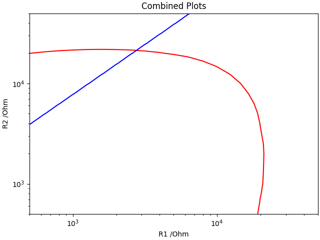
So I have the overlap, and it’s at a (R1, R2) point of (2k7,21k).
The beauty of this is if I want to improve my model of the diodes, or change the opamp in the circuit used it’s easy enough to repeat this analysis. The only faffy thing would be to adjust the frequency range / simulation run time to encompass enough time for the model. However given I’ve got a good base and any changes will (hopefully) have only minor impacts it’ll probably be fine.
The .asc files is here: sawtooth_generator.asc.
The code for anyone interested:
#!/usr/bin/python3

'''
This is a parser for the LTSpice sawtooth_generator.asc simulation.
Run it as a command with an arguemnet, eg:
`./log_parser.py sawtooth_generator.log`
'''

import re
import sys
import numpy as np
import matplotlib.pyplot as plt
from matplotlib import cm
import math

search_term = "\.step"

r1vals=[]
r2vals=[]
meas_list=[]
meas_name=[]

## Getting the R1 and R2 Values
# Parting the text
for lineno, line in enumerate(open(sys.argv[1],'r')):
    if re.search(search_term, line):
        #print(line)
        splitline=line.split(" ")
        r1=float(splitline[1].split("=")[1])
        r2=float(splitline[2].split("=")[1])
        r1vals.append(r1)
        r2vals.append(r2)
    if re.search("Meas", line):
        #print(lineno, line)
        meas_list.append(lineno)
        meas_name.append(line.split()[-1].strip())

#print(meas_list[1])
#print(meas_list[0])

meas_cnt=meas_list[1]-meas_list[0]

noofmeas=len(meas_list)

## Getting the Measurment data
meas1=[]
meas2=[]
meas3=[]
meas4=[]

for lineno, line in enumerate(open(sys.argv[1],'r')):
    if meas_list[0]+1 < lineno < meas_list[0]+meas_cnt-1:
        meas1.append(float(line.split()[-1]))
    if meas_list[1]+1 < lineno < meas_list[1]+meas_cnt-1:
        meas2.append(float(line.split()[-1]))
    if meas_list[2]+1 < lineno < meas_list[2]+meas_cnt-1:
        meas3.append(float(line.split()[-1]))
    if meas_list[3]+1 < lineno < meas_list[3]+meas_cnt-1:
        meas4.append(float(line.split()[-1]))

real_meas_cnt=len(meas1)

## Calculating the values of interest
periods=[]
freqs=[]
drs=[]

for i in range(real_meas_cnt):
    prd=meas3[i]-meas1[i]
    if meas1[i]<meas2[i]:
        # Rising edge of Vint came first
        ## MEAS1, MEAS2, MEAS3, MEAS4
        t1=meas2[i]-meas1[i]
    else:
        # Falling edge of Vint came first
        ## MEAS1, MEAS2, MEAS3, MEAS4
        t1=meas4[i]-meas1[i]
    freqs.append(1/prd)
    #reqs.append(math.log10(1/prd))
    #t1=meas2[i]-meas1[i]
    drs.append(t1/prd)

# Number of Unique Values
#(len(set(r1vals)))
#(len(set(r2vals)))

#converting to np arrays
r1array=np.array(r1vals)
r2array=np.array(r2vals)
drsary=np.array(drs)
frqary=np.array(freqs)

#convreting to meshgrid
r1mesh=r1array.reshape(len(set(r1vals)),-1)
r2mesh=r2array.reshape(len(set(r2vals)),-1)
drmesh=drsary.reshape(len(set(r2vals)),-1)
frmesh=frqary.reshape(len(set(r2vals)),-1)

## PLOTTING

# Setting up variables for simplicity
X=r1mesh
Y=r2mesh
fZ=frmesh
dZ=drmesh

# Key Levels
#flevel = math.log10(1000000/26.4) #frequency level
flevel = 1000/26.4 #frequency level
dlevel = 128/1056 #Duty ratio level

# Asthetic shiz
theme=plt.cm.bone


# Plot 1: Frequency Plot
fig1, ax1 = plt.subplots(layout='constrained')
CS1a = ax1.contourf(X, Y, fZ/1000, 10, cmap=theme)

CS1b = ax1.contour(CS1a, levels=[flevel], colors='r')
ax1.clabel(CS1b, fmt='%2.1f', colors='w', fontsize=10)

ax1.set_title('Frequency of Sawtooth')
ax1.set_xlabel('R1 /Ohm')
ax1.set_ylabel('R2 /Ohm')
ax1.set_xscale('log')
ax1.set_yscale('log')

# Make a colorbar for the ContourSet returned by the contourf call.
cbar1 = fig1.colorbar(CS1a)
cbar1.ax.set_ylabel('Frequency / kHz')

# Add the contour line levels to the colorbar
cbar1.add_lines(CS1b)
plt.draw()


# Plot 2: Duty Ratio Plot
fig2, ax2 = plt.subplots(layout='constrained')
CS2a = ax2.contourf(X, Y, dZ, 10, cmap=theme)

CS2b = ax2.contour(CS2a, levels=[dlevel], colors='r')
ax2.clabel(CS2b, fmt='%2.2f', colors='w', fontsize=10)

ax2.set_title('Duty Ratio of Saw Tooth')
ax2.set_xlabel('R1 /Ohm')
ax2.set_ylabel('R2 /Ohm')
ax2.set_xscale('log')
ax2.set_yscale('log')

# Make a colorbar for the ContourSet returned by the contourf call.
cbar2 = fig1.colorbar(CS2a)
#cbar2.ax.set_ylabel('R')

# Add the contour line levels to the colorbar
cbar2.add_lines(CS2b)
plt.draw()

# Plot 3: Combined
fig3, ax3 = plt.subplots(layout='constrained')
ax3.contour(X, Y, fZ/1000, levels=[flevel],colors='r', label="Freq")
ax3.contour(X, Y, dZ, levels=[dlevel],colors='b', label="DR")
ax3.set_title('Combined Plots')
ax3.set_xlabel('R1 /Ohm')
ax3.set_ylabel('R2 /Ohm')
ax3.set_xscale('log')
ax3.set_yscale('log')

plt.show()
This is surprisingly not always the case. Sometimes it’s a simulation thing, sometimes the circuit is broke, but we’ll take the win here.↩︎
Notice the {R1} and {R2} values? Also added meas statements as some sort of way of getting the data out.↩︎
There’s probably a way to parse the other output files, but when you’re a text hammer all problems look like parsing nails.↩︎
Well, actually it took a little faffing with some of the rising and falling triggers, but it’s good to ensure you’ve got what you think you have.↩︎